Pages

Signed integers addressing downsides..


  It isn't uncommon to hear things like "you should always used signed integers" from some developers. 

Well here is one downside of signed integers that bit me with regards to performance.

I had some SIMD code that needed to do some strided 64 byte loads. 

The actual code is more complex, but here is a simplified version to demonstrate.


_m256i StridedLoadsSigned( i64* p, __m128i adr){
     /*alignas(16)*/  int Mem[4];
    _mm_store_si128((__m128i*)Mem,adr);

    i64* low = p + Mem[0];
    i64* b = p + Mem[1];
    i64* c = p + Mem[2];
    i64* high = p + Mem[3];
    __m128i v = _mm_loadl_epi64((const __m128i*)(low));
    __m128i v3 = _mm_loadl_epi64((const __m128i*)(c));
    __m128i v2 = _mm_insert_epi64(v, *((i64*)(b)+4), 1);
    __m128i v4 = _mm_insert_epi64(v3, *(i64*)(high), 1);
    __m256i a = _mm256_setr_m128i(v2,v4);
           
    return a;
} 


Here is the horror story MSVC generates for this:


      vpextrd eax, xmm1, 3
        movsxd  r8, eax
        mov     r9, rcx
        vpextrd eax, xmm1, 2
        movsxd  rdx, eax
        vpextrd eax, xmm1, 1
        vmovq   xmm0, QWORD PTR [rcx+rdx*8]
        vpinsrq xmm3, xmm0, QWORD PTR [rcx+r8*8], 1
        movsxd  rdx, eax
        vmovd   eax, xmm1
        movsxd  rcx, eax
        vmovq   xmm0, QWORD PTR [r9+rcx*8]
        vpinsrq xmm1, xmm0, QWORD PTR [r9+rdx*8], 1
        vinsertf128 ymm0, ymm1, xmm3, 1    


According to UICA It has a predicted throughput of 14 cycles and issues 19 uops(Skylake)

 Now lets do one tiny change and make Mem unsigned. 


unsigned int Mem[4];


                vpextrd edx, xmm1, 2
                vpextrd r8d, xmm1, 3
                vmovd   eax, xmm1
                vmovq   xmm0, QWORD PTR [rcx+rdx*8]
                vpinsrq xmm3, xmm0, QWORD PTR [rcx+r8*8], 1
                vmovq   xmm0, QWORD PTR [rcx+rax*8]
                vpextrd edx, xmm1, 1
                vpinsrq xmm1, xmm0, QWORD PTR [rcx+rdx*8], 1
                vinsertf128 ymm0, ymm1, xmm3, 1


So what is the difference, and why is the 2nd one so much simpler? Well the compiler no longer felt the need to insert sign conversions, which preserves the sign of the 32 bit integer into the 64 bit address.


A further amusement is that this simplified code is basically the equivalent of _mm256_i32gather_epi64, but gather is implemented so poorly on most CPUs that this code will outform the hardware gather.

  On Zen2 _mm256_i32gather_epi64 emits 32 uops! 

The only CPU that I am aware of that might be better off with hardware gather is Raptor/Alder Lake P core(7 uops), unfortunately those are paired with E cores where gather is *terrible*(54 uops). Even modern Zen4 still has a fairly terrible gather(24 uops).


Bounds Culling: xyz vs morton vs hilbert


Here is a screen shot showing a debug mode in the game that renders the bounding boxes for edits near the player.

As you can see there are many of them, and this is in a relatively small area.

Even  a small world can end up with millions of these edits.

Now imagine you want to query a region of space that is quite large, perhaps 1km across!  

First we compile a copy of the world that overlaps the 1km bounds.

 This is our program we can run to evaluate the SDF within that bounds, we did manage to remove everything outside the bounds, but we still have an extremely large program...

 Now we need a second culling system! This one runs during the evaluation of points.  


 How it works 

The way in works in the game is that we also generate a list of instruction AABBs, these get stored in a SIMD friendly structure.  For culling if we find that none of our points overlap the bounds, we skip the program instruction range it would have otherwise evaluated.  

Evaluating every point against every instruction AABB would be slow and defeat the purpose of this, so multiple coarse layers are used.

 The first layer takes in our SIMD WIDTH * 32 (So for AVX2 this is 8*32=256) points, and computes a single AABB that contains all of them

  Once we have this first coarse point AABB, we loop over all instruction AABBs, and process them N at a time with SIMD.  This generates a 1 bit mask per instruction AABB.

 If there was an overlap, the we enter the second layer.

 This is a more refined culling process where it checks the SIMD_WITH points against that specific instruction AABB, it does this for all 32 loops and outputs 1 bit for each. 

This results in a 32 bit mask, if a bit is on we must process that SIMD_WIDTH set of points, if all bits are 0, we can skip all 256 points.  This results in a loop that operates using BitScanForward/zero lowest bit, rather than the traditional iteration from 0 to 32.

 The instructions bounds also have a similar bit mask that allows for skipping up to 64 bounds at at time with BitScanForward.


Results

(this was written before I added the 2nd layer so it is slightly out of date, with the 2nd layer the culling is more accurate and would show even better results than this)

 Now given that most evaluations aren't processing one point, but hundreds to thousands at a time, and our culling is somewhat coarse(N = multiples of 32) because we don't wish it to dominate program time, does the order in which the points are passed in matter? Well yes, yes it does.

 The default order is more or less xyz, with some psuedo randomness just based on whatever the program happened to do to spit the points out. This is not a great order, and results in significantly more bounds overlaps being true.

 Anyway I instrumented the program and aggregated the *not* culled rate using xyz, morton and hilbert. 

Here are the results, lower being better.

  • xyz         .222
  • Morton  .1159
  • Hilbert   .09

While these numbers don't look too different, keep in mind the speedup is relative, so going from xyz to hilbert is .222/.09 =  2.5x, I'll take that!

The speedup for morton to hilbert is 1.287x, I also find this to worth the extra cost(hilbert is about 4x slower to compute, but computing the indices isn't a huge factor).

The morton/hilbert approaches do require sorting, and generating the respective indices, thankfully I have SIMD optimized code for this, so the cost is pretty minor.

I am enabling this dynamically based on the number of bounds, once it goes over a certain threshold Hilbert order is imposed.


Displacement Format


 I'm changing the displacement map format. 

The current format is a histogram normalized u8, generated from the source maps which are u16.

When zooming in there simply isn't enough precision and we start to see stair stepping from the u8


So the format I am switching to is roughly based on BC4, but as I'm decoding on the CPU I decided to simplify it. 

BC4 stores per 4x4 pixels a min and max value, and a 3 bit interpolation weight per pixel. The total size is 64 bits per 4x4 block, half of u8.

First I removed the 2nd mode, where the order of min/max is swapped, this simplifies the decoder.

Second I changed it so that rather than storing a min and max value per 4x4, we store a min and ratio between min and 255. 

This changes the precision range from 3-11 to 3-19 bits and is only possible because I removed the 2nd mode.

Third I changed the way the indices are stored, so that 0-7 maps directly to the lerp ratio. 

I have no idea why BC4 stores it indices in such a random order, but it makes it much harder to decode on the CPU.

I'll refer to my format as DBlock.

 I wrote a fail fast test compare the DBlock vs U8 encoding,  one immediate downside of DBlock is that the decoder requires more instructions than U8.  On the other hand the total memory is half, so less cache misses. Also the blocks are in 4x4 format which is essentially a partial morton order, so again better cache access patterns.

Visually DBlock wins in virtually every case despite being half the memory. This is because the vast majority of 4x4 blocks are better captured by a local gradient encoding.  In theory for blocks that contain large differences between min/max DBlock should look worse, but I am not easily able to spot the difference.

The only real downside is the complexity of the decoder, in particular with U8 I was taking advantage of that fast that I could load multiple pixels with a single gather. This is far more difficult with DBlock, since each "pixel" is now 4x4 pixels,  and 8 bytes in size. 

Also this is all SIMD based, I don't have scalar decoders. 

Thus branching on whether the X coordinate crosses from one block to another doesn't work well, it is very likely at least one of the lanes will cross blocks.

 The initial decoder simply does many more gathers than the U8 one, for a 2x2 bilinear sample the U8 decoder required 2 gathers, with an extra 2 only when the X coordinate wrapped around(Repeat sampling).  

The initial DBlock decoder for bilinear requires 8 gathers(in best case theoretically we only need 1 or2, but worst case is 8), although in many cases they are gathering from the same block, so it should be possible to eliminate some of these once I write a more optimized decoder.

 One interesting thing is that for quadratic sampling(3x3), DBlocks number of gathers doesn't change from bilinear, and we can get everything we need with 8.

 One perf improvement I quickly added was to switch the gathers to 64 bit sized rather than 32 bit, as our blocks are 64 bit, and 64 bit gathers do run faster.

 Another option would be to drop the gathers and use 128 bit loads per lane, then shuffle everything around. I'll probably test this at some point, but it is a large # of instructions, so it may not be a win despite dropping the gathers.


*Update: I wrote the 128 bit load/swizzle based version and it does outperform the gather based implementation, and is now the default version. This is on Zen2, where gather is particularly slow and decodes to an obscene number of Uops.


Future: At some point I'd like to port the volumes to also using this format (Edit: this has been done although it is a slightly different format since it targets 3D blocks)


Profilers I use

Visual Studio Profiler

The profiler built into Visual Studio is a sampling profiler.  When you examine a function, it can display a per line cost, although it is often off by a 1, and the real cost was in the previous line. 

 I find this profiler mostly useful to look for hot functions, and to get an approximate breakdown of the cost within these functions. On the other hand it has no idea about when and where context switches occurred, and so can sometimes be incorrect. 

A benefit for this profiler is that is display the data directly within Visual Studio, an unfortunate thing I've noticed with some profilers is that the visualizer uses a custom code editor and it looks awful(Intel Vtune..)

Tracy

This profiler is a hybrid frame/sampling profiler. 

For the frame based part you need to instrument your program with scope based macros, giving each section a name.  You can also instrument many other things such as threads, memory allocations, and mutex acquisition. 

 It uses a separate tool to visualize the data, which allows inspecting each frame individually, or to aggregate a given function, viewing statistical data about it.

 One very nice feature of Tracy is the fact that it is context switch aware, although you do need to run Visual Studio in admin mode so Tracy can acquire the necessary information at runtime.  

 When enabled this greys out the threads that were inactive, this way what appears to be a random long running tasks, is clearly just a task that was context switched out.

 One thing I didn't care for was the amount of bloat in the tracy header file, so I created by my forward declarations/macros/functions to wrap it, to avoid including so many heavy headers.


Visibility Buffer

 I rewrote the main render to use a visibility buffer, if you are unfamiliar with this, it is a renderer whose first pass has a very simple pixel shader that writes out the draw call ID & triangle index.

Given the high triangle count I figured the visibility buffer would perform better since it cancels out much of the 2x2 overshade issue that arises with tiny triangles, and this turned out to be very correct. 

The game now runs significantly faster, and is also much more portable, as I don't have to rely on driver extensions to get access to barycentrics.

 My visibility buffer is 32 bit, 14 bits for the triangle ID, and 18 for the draw call ID.  This did require limiting triangles counts to 14 bit, which was not an existing requirement, but was simple enough to add.


Normals maps into HemiMaxn

 I switched the normal maps from using euclidean xy to using hemi maxn, this is a hemispherical encoding I came up with that is somewhat similar to HemiOct.  


 This provides higher quality, with only a few extra instructions required to decode.


I also created a variant for a full spherical view, it is 2x as wide as it is tall.


Here is spherical maxn used for a skybox, this shows a 360 view.  I generate this by projecting the primary screen render onto the maxn view, then warping it forward as the player moves around. This is used as the basis for the environment map. It does get distorted if the player never turns their head, so I'll probably need to add a specific pass to render a low res version behind the player occasionally.

Camera with Signed Distance Field

 The camera uses the local SDF to guide itself, attempting to stay at least a fixed distance away from the nearest surface, while also avoiding obstructions that may be blocking the view of the players body.  

When moving away from a surface it uses the gradient of the SDF to determine the direction to move in. 

It also computes the lipchitz bounds to accommodate and correct for bad distance fields.

 The player also moves using (semi) camera relative controls, so the movement of the camera needs to be very smooth and predictable. 

  The design uses two virtual arms, one extending upward from the players body, and the 2nd, connected to the top of the first, extends backward. Left/right with mouse spins the first, while Up/Down moves the 2nd. It feels like a first person camera while actually being third person.

I apply temporal smoothing in a few places to prevent jittery behavior.


Network model

A brief overview of how networking is implemented in the game.

UDP is the protocol, with a custom reliability/ordering capability available.

Packets are compressed with zstd using a dictionary.

The game sends all input events to the server, these are then resent out to all other players, who replay them in the correct order.

Physics data is constantly sent out by the server, and clients interpolate toward the servers version. It uses a priority system to determinate which bodies to transmit, the system is stateless and relies on weighed randomness to determine which is sent. Basically compute a weight per body(based on proximity/visibility etc) + a random value between 0-1 for each body, multiply them, and then pick the top N bodies.  

I experimented with extreme quantization of physics data but found it caused jittering, so the quantization is limited to 16 bit floats, the server imposes this same quantization on its own data to match the clients.

 Map data is the bulk of what is initially sent, basically all those damn edits! The server tracks exactly which edits each player is aware of, when a player connects it bulk sends sections of the world to the player. And as minor edits happen these are also send out to players with some location priority to pick the most important. Edit order matters so each edit has an associated order so they can be reassembled in the correct order.


Quasi Virtual Texturing System


This is an overview of a quasi virtual texturing system that I implemented for my game.

I use this system instead of a traditional virtual texturing system for the following reasons.

  1. Supports all levels of anisotropic/trilinear filtering, even on old hardware
  2. Doesn’t use tiled resources which require newer GPUs, and aren’t available on Windows 7 with d3d11
  3. I use triplanar texturing exclusively, and do not have traditional UVs

Algorithm

This algorithm uses multiple texture arrays, and a structured buffer that indicates per material, which array to sample from.

It uses a fixed sized amount of memory for textures on the GPU.

Textures are limited to square powers of 2, the only sizes supported are 256,512,1024, and 2048. This reduces the number of arrays we will need to a reasonable number.

I pre-generated a texture array that contains all of the mips of size 256 and under, for all textures.

I also allocate fixed sized arrays for 512,1024 and 2048; with the larger sizes having progressively fewer slots.

Number of slots : Here are the number of slots I have per array, these numbers are mostly arbitrary.

  • 256: # of textures
  • 512: 128 slots
  • 1024: 32 slots
  • 2048: 8 slots

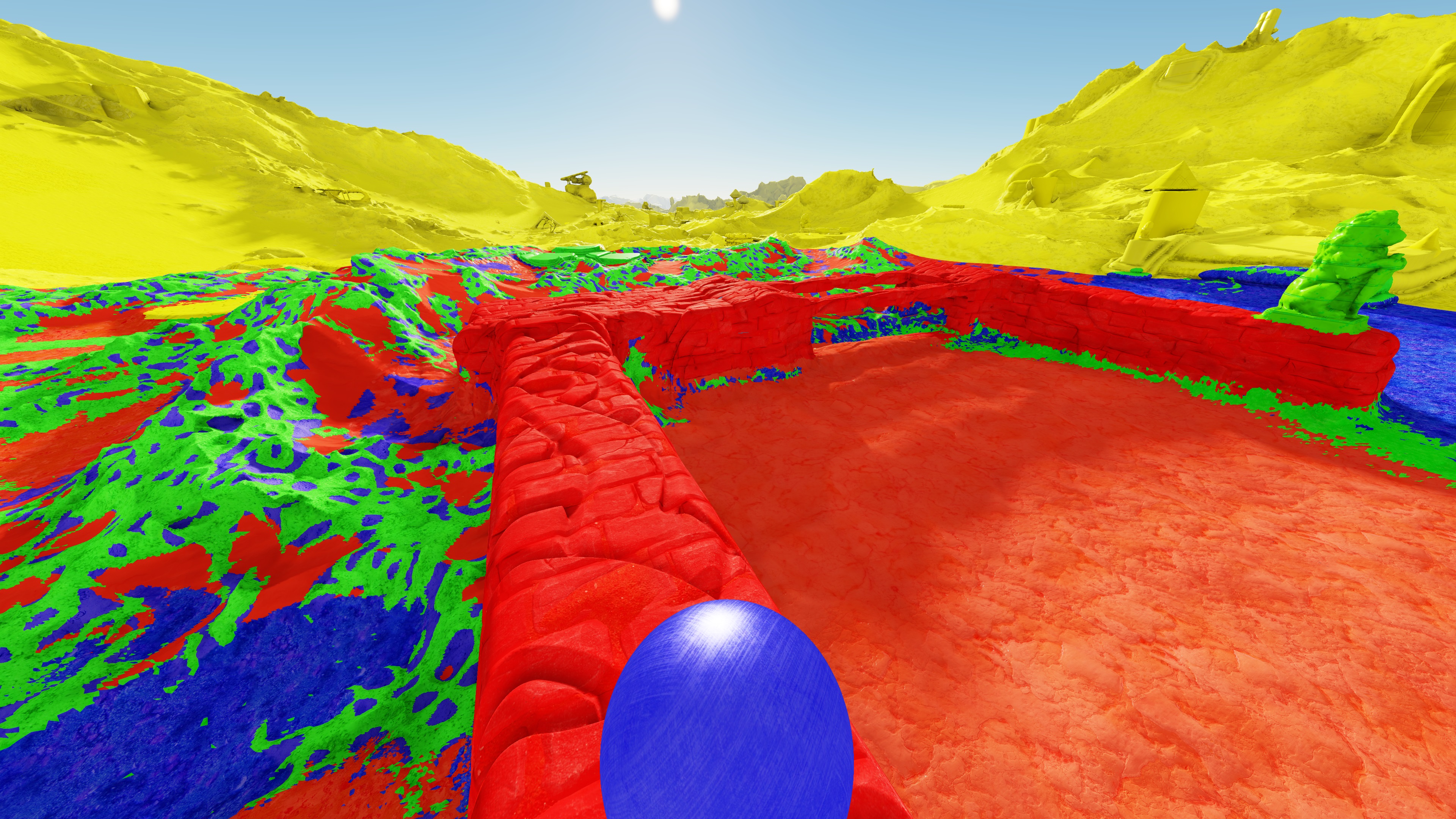
Here is a visualization of the arrays.

SDFShape2 

 Yellow is 256, Green is 512, Blue is 1024, and Red is 2048.
I force everything to use 256 past a certain distance to reduce divergence

A structured buffer is used as an indirection mapping; pass in the material ID, and retrieve which array to sample from, and which slot in the array.

Prioritizing Textures

As there is a limited number of high resolution textures that can be on the GPU at any given time, a system to was needed to determine which textures should be resident.

This is done by storing the N most important textures, along with a score, for each voxel patch.

The score is simple the number of vertices that reference the texture.

Each frame, for visible patches, the score is added to the appropriate textures/MIP based on the distance from the camera for the patch.

Patches which are out of the frustum or occluded do not get added.

The textures/mip with the highest score, that is not resident on the GPU is then considered for uploaded, if it has a higher score than a resident texture at the same mip level.

Only one texture is uploaded per frame, to limit the amount of data that needs to be transferred.

The structured buffer is also updated to reflect where the GPU can find the texture.

Latency is reduced by having the CPU side also store a cache of recently accessed textures, the caches size is adjustable, but is currently set to 300mb.

Results

The system works well and transparently pages in texture data based on visibility.

It never suffers from horribly blurry textures since the 256 mips are always available as a fallback.

Even standing still and turning the camera around can and will cause textures to be paged in/out.

Limitations

  • D3d11 has a max texture array size of 2048. This means this system can only support 2048 separate materials. I am nowhere near this limit, so this isn’t an issue for me.

GPU Texture Format for PBR

Visuals with PBR.  


Objective: encode a full PBR set of channels into as few bits as possible, with good performance.

From testing it appears that each additional texture adds significant cost, using 3 textures to encode the PBR signal with a size of 2 bytes per texel is much more costly than 2 textures at the same overall number of bytes per texel.

The PBR system I'm using has 8 channels:

3 base color
2 normal 
1 roughness
1 metallic
1 AO

 If we attempt to store the normal in BC5, a two channel format designed specifically for tangent space normals, we have 6 channels remaining, and cannot fit that into a single texture, as none of them support more than 4 channels.
So we cannot use BC5.

 There are two good options I've found instead, both using the same layout, two textures, both with 4 channels.
  
On anything D3D11 and newer, BC7 can be used.
For pre-D3D11 systems, BC3 textures can be used instead. 

The normal will be split and stored into the alpha channels, which should help preserve precision of the normal.

Texture1: RGB: base color A: normal.x 
Texture2: RGB: ao, roughness, metallic.  A: normal.y 

*Texture1 can be safety set to SRGB, as both BC3 and BC7 treat the alpha as linear.

Uncompressed signal: 8 bytes 
Compressed: 2 bytes in both BC3 and BC7 formats

Encoding speed:

Using AMD Compressonator BC3 is fast to encode, even with quality set high it churn through BC3 fairly quickly.

Another encoder I tested was Crunch, a BC1/BC3 compressor that applies a lossy entropy reduction algorithm on top of the lossy block compression algorithm- this enables crunched BC1/3 files to compress much smaller on disk.
I decided not to use it because the compressor was very slow, and I feel that BC1 already looks less than stellar(the endpoints are 565..)-- throw in even more artifacts from Crunch and the textures just didn't look very good.


AMD Compressonators BC7 encoding is not nearly as fast as its BC3. 
This is understandable as the format is vastly more complex.

With the quality set to low, it still takes much longer than BC3 at high quality. 


BC format Impact on Rendering
There is no observable difference in rendering performance between BC3 and BC7 on my AMD 280x.  
Both are observably faster than uncompressed, not surprising given that uncompressed is 4x larger.

BC3 vs BC7 Visual Quality: 

I have only run BC7 high quality on a few images, I'd probably have to run it overnight and then some to generate high quality BC7 for everything.

 Comparing low quality BC7 vs high quality BC3:

BC3's RGB part(identical to BC1), can only encode 4 possible colors in each 4x4 region, BC7 is far less limited.

For noisey images the difference isn't all that noticeable, but if you look closely BC7 generally has slightly more detail.

For anything with smooth gradients BC7 is clearly superior.

Normals:

BC3 has dedicated 8 bit end points and 3 bit indices for the alpha channel, while BC7 may or may not even have dedicated indices for alpha, as this is chosen on a per block basis. 

There is no obvious difference in the normals, but when I zoom in I can occasional spot areas where BC3 appears to have done a better job, but this is rare, and the overall improvements in the other channels is larger improvement than this small loss. Also running BC7 high quality may change this--

 Size on Disk: 
Both BC3 and BC7 are 8 bits per pixel
When bit compressed, in this case with zstd, the BC7 files are generally about 1-2% smaller.

I tried lzham(an LZMA variant), but the files are only about 5% smaller than zstd level 19, not worth the 5x slower decode.


Possible/Future Improvements:

1.  Quality of all channels can be improved by tracking min/max for the entire image and then re-normalizing it. This would require 2 floats per channel in the shader to decode though.

2. The normals in the normal map are in euclidean space, this wastes bits since some values are never used. Octahedral coordinates make better use of the available bits, and decoding isn't really much different.


Metal channel is active for many of the objects seen here


Adding SDF Collision to Bullet Physics


Bullet Physics is an open source physics engine that is sometimes used for games and movies.

It supports many near phase collision types such as spheres, boxes, capsules, triangle meshes and convex hulls.

None of these were a good match for my signed distance fields(SDF).

Triangle meshes might seem like a solution, but they have two obvious issues.

  1. No volume which leads to penetration issues and bad collision detection
  2. Uses lots of memory to store the mesh

Convex hulls might also seem like a solution, but also have a downsides

  1. They only work with convex data. To work with concave data you must generate multiple hulls and stick them together.
  2. Not very accurate representation of the original shape unless you stitch many of them together, this would be infeasible for the world/terrain shape which is many kilometres in size

So I decided to extend bullet to directly support SDF vs SDF collision.

As everything in my game world is represented by an SDF, I do not need any of bullets built in collision types and only use SDF vs SDF collision.

Collision Algorithm

The solution I went with is based on generating a point hull for the SDF, a point hull is a list of points that lie within the shapes negative space. In my implementation all points in a given hull uses the same radius.

To perform collision detection between two SDFs, you treat one of them as a point hull and the other as an SDF. You transform each point in the point hull into the space of the SDF and sample the SDF. If the distance to the negative space is <= the point hulls radius, you have a collision.

I decide which object will act as the point hull based on who has the smaller point hull radius, this ensures consistent collision, and allows for the smaller object to collide against the larger objects full SDF.

For the world/terrain shape I disable the point hull generation pass, it is always treated as the SDF when colliding.

For points that are found to be colliding, a second pass is run to generate the normal and collision depth, and to reduce the number of impact points down to four(this is the number of points bullet wants fed to it).

Result

SDF vs SDF supports both convex and concave shapes.

It also has fewer issues with penetration than triangle meshes since SDFs have proper volume, even if a small object penetrates into a larger one, it will still be pushed out in the correct direction.
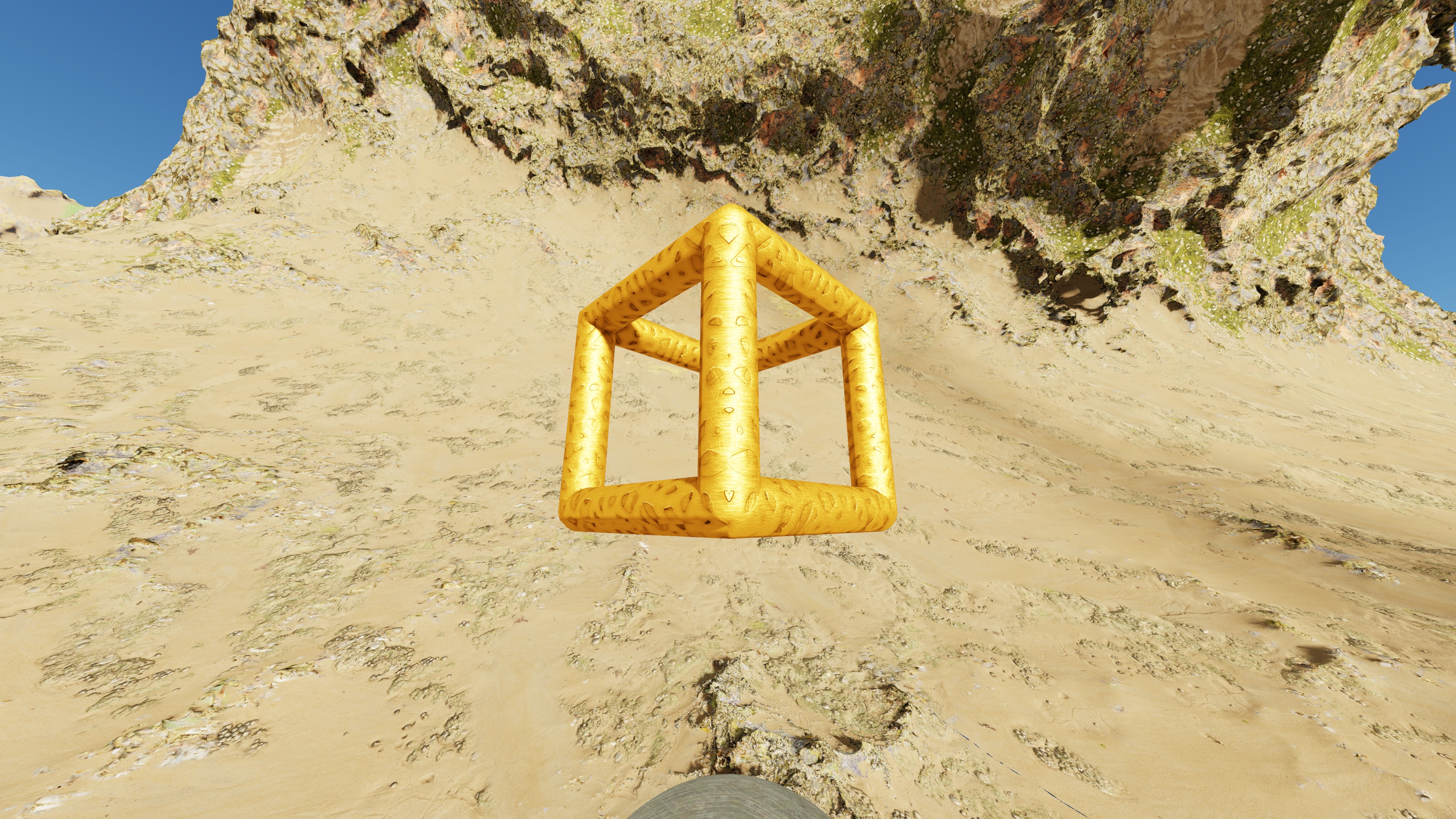
SDFShape1 

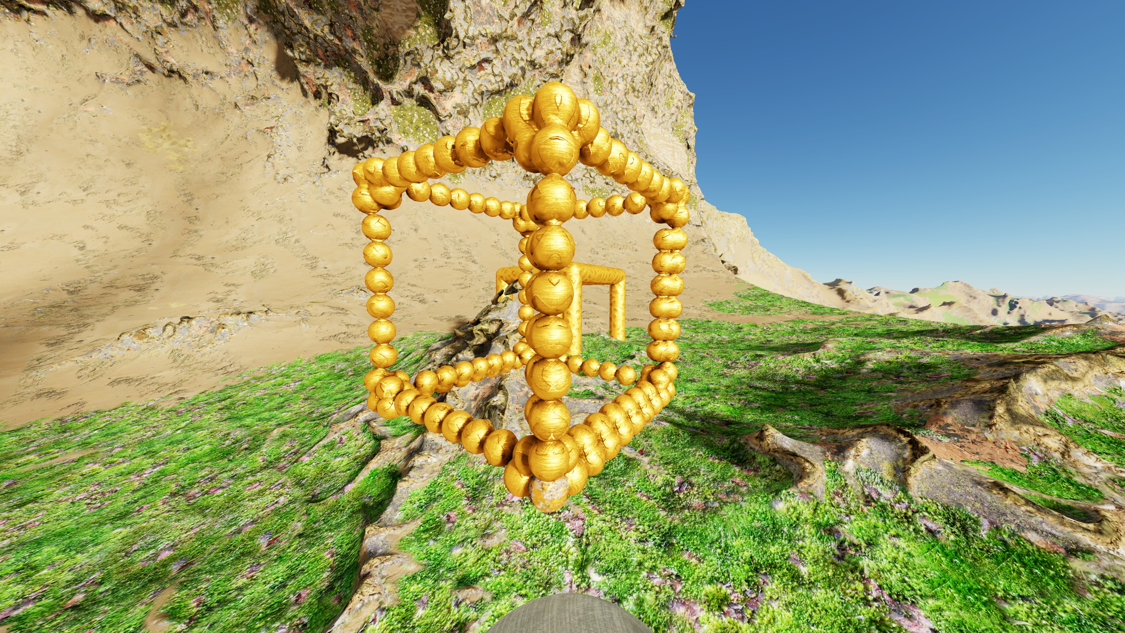
Here is a shape for which we will generate a point hull
SDFShape2

And here is a visualization of the point hull.

Optimizations sometimes known as midphase

There are numerous ways to optimize this, but here are some that I use. The underlying SDF algorithms are already all SIMD, so this is focused on algorithmic optimizations.

Surface Approximate

Instead of sampling the full SDF against all of the points, I first run a pass that only samples eight points on the point hulls AABB within the SDF. It then uses those eight points to perform a quick rejection of points that incapable of colliding because they are too far away. This often eliminates >90% of the points, so we can skip full SDF evaluation.

Temporal Collision Frame

This is a frame that is specific to a given object vs object collision, it records a rough approximation of the previous collision attempt between the two shapes. If not enough movement or rotation has occurred it can early out and skip performing the full near phase–the previous contact points are reused.

Handling SDFs with broken distance formulas

Otherwise known as Lipschitz continuous– we want gradients whose magnitude is as close to 1 as possible.

Some SDFs do not have euclidean correct distances, for these cases I run a fix up step which calculates a correction factor based on the rate of change in the local space of the SDF.

My correction algorithm takes the distances calculated for the AABB of the point hull projected into the SDFs space, and compares the true distance between the points against the distance returned by the SDF. It compares all of the points against each other, and uses the largest ratio of (sdf distance/true distance) as the correction factor.

This allows for colliding against fractals and other complex formulas, which often have incorrect distance formulas.

Performance Notes

In scenes with many moving & colliding objects:

Initially my SDF near phase and Bullets solver were about equal in cycle usage.

After adding various optimizations to reduce the time spent in the SDF near phase, the solver is now the primary waster of cycles.

Bullets solver has a few SSE based implementations, but they are AoS not SoA based, so the performance gain is minimal.

Bullet has a few inefficiencies in how it works, it loves to iterate over every single CollisionObject just to access a single bool, while this is not a problem for small scenes, it does not scale to the number of physics objects I plan to use.

I plan to rework this part of Bullet in my local copy, and have already rewritten/removed a few passes Bullet was performing that I did not need.

Pseudo Continuous Collision Detection

Bullet has some support for CCD(Continuous Collision Detection), but I’m using my own pseudo CCD instead.

My CCD solution is very simple:

Calculate the maximum distance an object can travel in a given physics tick based on its current velocity, and expand the point hulls radius to incorporate it.

At high speeds this causes expansion, but I cannot visually tell that this is happening.

I run physics at 120 hertz, but I did test it at 60 hertz and it seemed to work fine there also.

I’m not currently incorporating angular velocity, but I will probably add that at some point.

Future Work

  1. The algorithm for placing points within the hull could always use more work.
  2. It might also be worth looking into storing a per point radius, this will allow for less points in some situations
  3. Angular Velocity for CCD
Higher Quality Vertex Normals

 I use the Oct16 format to encode my vertex normals, this format is two 8 bit channels in octahedral mapping.

  Most of the time this was sufficient, but under certain conditions artifacts were visible-- such as the surface of a smoothly varying sphere using triplanar texturing, whose weights are based on the normals.


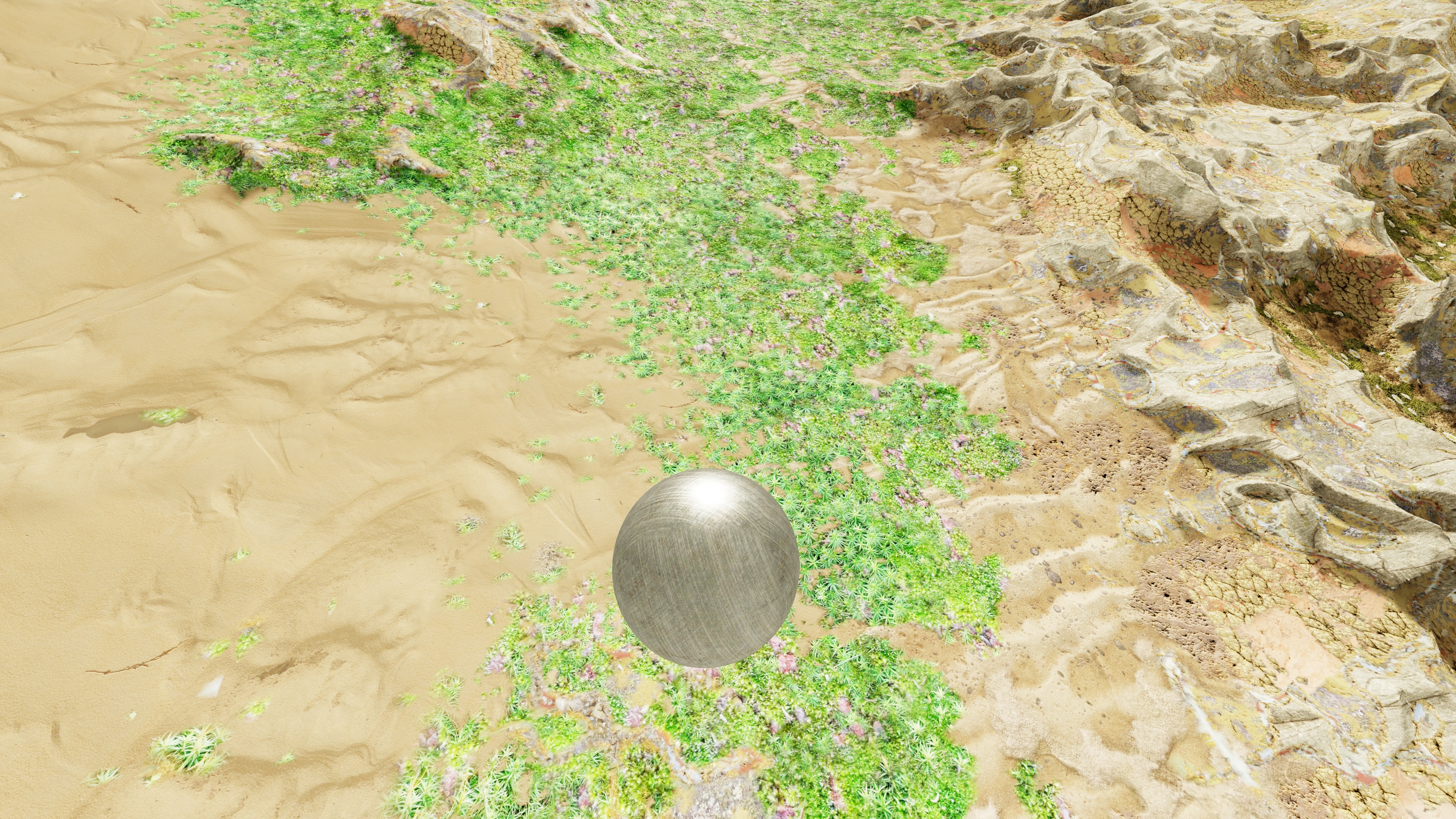
Here is a visualization of the Triplanar weights generated from the Oct16 normals.


There is a very obvious diamond pattern visible.
Even switching to Oct20(10 bits per channel) does not completely solve this, the diamonds are much smaller, but they persist.


Oct16, but with custom scale/bias


Instead of adding bits, I decided to take advantage of the fact that most triangle patches only use a
limited range of the world space normals.

I track min/max per channel for the entire patch, then encode the normals so that the full range of bits is used.

Decoding in the shader requires a custom scale and bias parameter per channel(4 floats for the two channel Oct16).

There are no extra instructions,  as a fixed scale of 2 and bias of -1 was previously being used to transform from [0,1] to [-1,1] range.


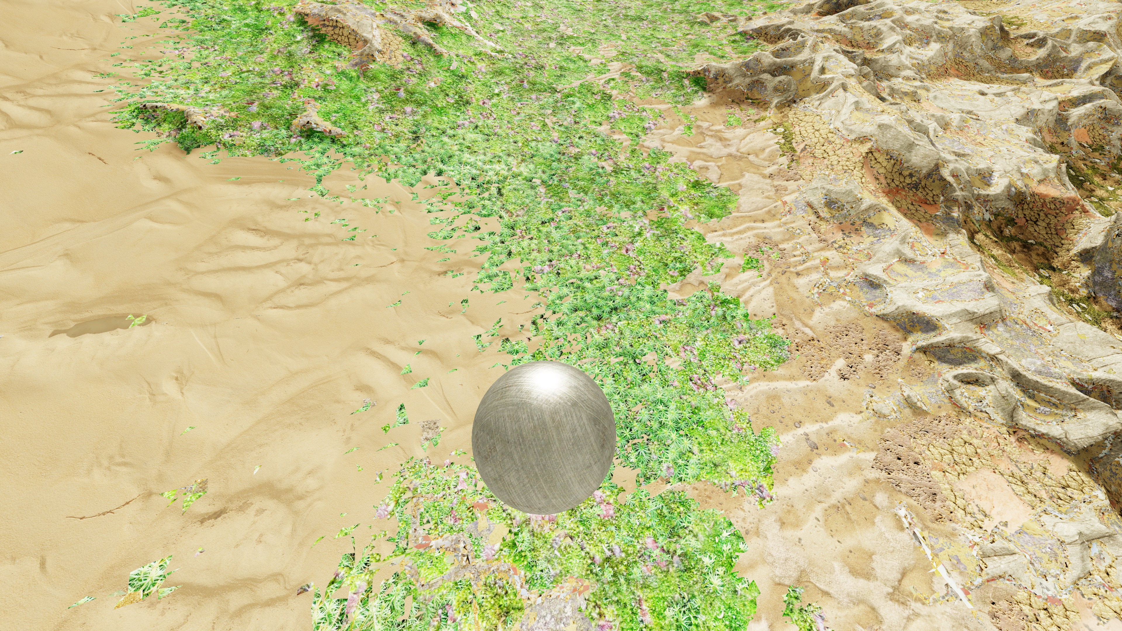
The 2nd image was encoded this way, the normals are still using Oct16, so only 16 bits per normal, but with a custom scale/bias per patch.

 In the majority of cases this provides many extra bits of precision, and in the worst case it degrades back to standard Oct16.

Faster Triplanar Texturing

Here is a method I created to improve performance when using Triplanar texturing.
I also think it looks better.


So the standard triplanar texturing algorithm you will find in varous places on the internet looks something like this.

float3 TriPlanarBlendWeightsStandard(float3 normal) {
float3 blend_weights = abs(normal.xyz); 
blend_weights = (blend_weights - 0.55);
blend_weights = max(blend_weights, 0);   
float rcpBlend = 1.0 / (blend_weights.x + blend_weights.y + blend_weights.z);
return blend_weights*rcpBlend;
}

If we visualize the blend zones this is what it looks like.


Red/Green/Blue represent one texture sample.

Yellow/pink/cyan represent two textures samples.

And in the white corner we need all three.

As we can see the blend width is not constant, it is very small in the corner and quite wide along axis aligned edges.

The corner has barely any blending as we have pushed our blend zone out as far as possible by subtracting .55.(anything over 1/sqrt(3) or 0.577 results in negative blend zones in the corner).

This results in needless texture sampling along aligned edges, stealing away our precious bandwidth.

Constant Blend Width


What we want is something more like this-- constant blend width.

We do this by working in max norm distance instead of euclidean,  as our planes are axis aligned anyway--

Here is the modified code that generates this:
float3 TriPlanarBlendWeightsConstantOverlap(float3 normal) {

//float3 blend_weights =  abs(normal);
float3 blend_weights = normal*normal;
float maxBlend = max(blend_weights.x, max(blend_weights.y, blend_weights.z));
blend_weights = blend_weights - maxBlend*0.9f;

blend_weights = max(blend_weights, 0);   

float rcpBlend = 1.0 / (blend_weights.x + blend_weights.y + blend_weights.z);
return blend_weights*rcpBlend;
}


 You can adjust the blend width by changing the scalar .9 value.

On my GPU the constant version runs slightly faster, likely because there are less pixels where more than one texture sample is required.

I believe it also looks better--as there is less smearing along axis aligned edges.


Here is a shadertoy I created if you want to play with it


Barycentric Coordinates in Pixel Shader

 EDIT: this is out of date, it is better to use visibility buffer and manually calculate barycentrics

Recently I was in need a way to perform smooth blending between per vertex materials.

Basically I needed barycentric coordinates + access to each vertices material in the pixel shader.

Unfortunately this isn’t built into the common rendering APIs, and so requires some extra effort.

Here is a list of some possible solutions:

Geometry Shader: Assign the coordinates: (1,0,0), (0,1,0), (0,0,1) to the vertices of the triangle. Also write the three materials to each vertex. This method is easy to implement but has terrible performance on many cards, since it requires a geometry shader. When enabled on my AMD card, FPS drops to half or less.

The following two methods are D3D11/12 focused

AMD AGS Driver extension: AMD has a library called AGS_SDK which exposes driver extensions, one of these is direct access to barycentric coordinates in the pixel shader. It also allows for direct access to any of the attributes from the 3 vertices that make up the triangle. This method is very fast and works well if you have an AMD card that supports it.

 float2 bary2d = AmdDxExtShaderIntrinsics_IjBarycentricCoords(AmdDxExtShaderIntrinsicsBarycentric_PerspCenter);
 //reconstruct the 3rd coordinate
 float3 bary = float3(1.0 - bary2d.x - bary2d.y, bary2d.y, bary2d.x);

//extract materials
 float m0 = AmdDxExtShaderIntrinsics_VertexParameterComponent(0, 1, 0);
 float m1 = AmdDxExtShaderIntrinsics_VertexParameterComponent(1, 1, 0);
 float m2 = AmdDxExtShaderIntrinsics_VertexParameterComponent(2, 1, 0);

Nvidia FastGeometryShader: Nvidia also have driver extensions NVAPI, and one of these is the the “fast geometry shader” for when you only need a subset of the features geometry shaders offer. It should be possible to use this to pass down barycentric coordinates & materials, but I do not have an Nvidia card to test this on.

Embed Into Vertex Data: Another option is to enlarge the vertex, and embed the barycentric coordinates and the 3 materials directly into it. This is probably a better fallback than the GS, although it does have the downside of reducing vertex reuse, since many vertices that were previously identical would now differ.

Domain Shader?: I haven’t tried this method, but I think it might be possible to pass down barycentric coordinates from a domain shader

Visual Comparison

BaryOn 

 Ground rendered using barycentrics to perform smooth blending between materials

BaryOff 

 Ground rendered without barycentrics, the material is selected from the base vertex and there is no blending between materials

AVX2 Gather


Masked Gather vs Unmasked Gather

  AVX2 has masked gather instructions(_mm_mask_i32gather_epi32 etc), these have two additional parameters, a mask, and a default value that is used when the mask is false. 

  I was hoping masked gathers would be accelerated, such that when most of the lanes were masked off, the gather would complete sooner, but this does not appear to be the case.

   The performance of masked and unmasked gathers was very similar, but masked gathers were consistently slower than unmasked gathers.


 Load vs Gather vs Software Gather

To compare gather with load, I created a buffer and run through it in linear order summing the values.
 I forced the gathers to load from the same indices the load was operating on.  Indices(0,1,2,3,4,5,6,7), incremented by 8 for each loop.

Software gather loaded each index using scalar loads instead of the hardware intrinsics.
Gather was generally ~1.2-1.5x faster than software gather.

 Performance was depended upon the cache level that buffer fit into.


Buffer fits in L1

Load is ~10x faster than Gather

Buffer fits in L2

Load is ~3.5x faster than Gather

Buffer greater than L2

Load tapers off to ~2.x faster than Gather


This was all run on a Haswell, newer chips might perform differently.


Moment of Inertia of a Distance Field

While adding physics support to my voxel engine I needed a reasonable accurate & fast method to calculate the moment of inertia, volume, and center of mass for an arbitrary distance field.

I've written this C++ code to do so.
Feed it a regularly spaced grid of points and distances.
The points must fully bound the negative space of the field to be accurate.

The common primitives, such as a sphere, there are established formulas that we can compare against.

For a 10^3 distance field of a sphere, the estimate is off by about 1%, close enough for me.
If more accuracy is needed, the sample rate can be increased.

SDF Based Occlusion Culling


I’m going to describe an occlusion culling algorithm I came up with about 4 or 5 years ago. I use it in my game and it has worked well for me.

If you do not know what occlusion culling is, it is culling objects that are in the frustum, but are blocked from the users view, and do not contribute to the scene.

Prior to this I used a Software Rasterizer based implementation, but I found that it was problematic for the following reasons.

  • Low resolution: not a huge issue, but it is much lower resolution than the GPU rasterizer so it isn’t completely correct
  • False Occlusion: since my occluders had to be auto generated at run time from arbitrary SDFs, I used a convex hull approximation which was not always conservative, this caused some false occlusion
  • Memory: each occluder had its own set of triangles that needed to be stored. Also meant jumping around in memory to access each of these sets.

SDF Occlusion Algorithm Overview

My scene is represented with triangular patches, each containing perhaps 500 to 2000 triangles. They are approximately equal size in screen space.

SDFShape2 

 I’ve scaled the patches down here so that we can see gaps between them

Basically we want to shoot rays from the viewers eye to each patch.

Because our scene is represented with a signed distance field, we always know the distance to the nearest surface.

If there is ever a point along the ray where we are inside of something, and the distance to the surface is sufficient to occlude our patch, we know the patch isn’t visible.

Optimizing to make it practical

The number of patches depends on the settings, but a typical number after frustum culling might be 10,000.

Shooting 10,000 rays through complex SDFs is quite slow, thankfully it is turns out that each frame is generally very similar to the previous, so we can take advantage of temporal stability.

Typically I only end up tracing around 100 rays per frame.

This is done by tracking previous occlusion results, and storing a sphere that represents the most occluded point.

The next time around, for patches that were occluded, we can quickly retest them without needing the SDF, by using a sphere occludes sphere test.

If that fails, we can still optimize by starting the ray test near the point of previous occlusion.

For patches that were previously not occluded, we can actually perform a fairly similar test, if there hasn’t been enough relative movement, there is no need to test the SDF, and we can assume the object is visible.

I differentiate between dynamic and static parts of the scene, as these temporal tests only work reliable for the static part.

I also use a timer to set a max time that this tracing process can run per frame.

Other Benefits

I track an occlusion ratio for each patch, this is between 0 and 1.

So even if something isn’t completely occluded I can still tell when it is partially occluded.

I use this occlusion ratio to adjust the priority for patch splitting and generation.

  • Patches that are completely occluded are never split.
  • Patches that are partially occluded, have a much lower score/priority, and won’t split until the user gets closer.

Future Work

Dynamic objects are occluded by static objects, but I haven’t yet added the code for dynamic objects to occlude anything. It isn’t terribly difficult, but I don’t think it will contribute much so I haven’t prioritized that work.

Potential downsides

  • While this algorithm works well for me, this is largely due to the precise way that may engine works, it is probably not well suited to a more typical game engine like Unreal which does not work based on equally sized in screen space triangular patches.
  • Thin objects don’t occlude as well as a software rasterizer based implementation, this is because it relies on the object having volume
  • Occluder fusion isn’t the best

Video of my Distance Field Engine

This is a short clip showing my engine. 
It uses distance fields to represent all geometry.
Don't confuse it with a minecraft like engine--those use 1 bit filled/not filled.
It is written in very SIMD heavy C++.


gflops on various processors


This is the execution engine for Haswell.

Port 0 and 1 can both execute FMA/FMul.

I'm going to write down general Gflops ratings for commonly used CPU's, broken down by how those numbers are calculated. This is mostly for future reference for myself.

Haswell i7 4770k at 3.5ghz.

8(AVX) * 2(FMA) * 2(two FMA ports) * 4(cores) * 3.5(ghz) =448 gflop

Kabylake i7 7770k: nothing much has changed here, but it is clocked at 4.2ghz.
It does have faster div/sqrt and fadd can run on two ports, but that is not reflected in flops rating.

8(AVX) * 2(FMA) * 2(two FMA ports) * 4(cores) * 4.2(ghz) =537.6 gflop

AMD chips support AVX/AVX2, but internally it only executes 128bits at a time.

Xbox One Jaguar AMD CPU:

4(fake AVX) * 2(ports) * 8(cores)* 1.75ghz  =112 gflops

AMD Zen CPU: the exact ghz isn't know, but demonstration had it at 3.4.
It supports AVX2, but breaks it into 2x4 SSE internally(half throughput of intel)

4(fake AVX2) * 2(FMA) * 2(two FMA ports I *think*) * 8(cores) * 3.4(ghz) = 435.2 gflop

Intel Skylake Xeon added AVX512 support, unfortunately it appears AVX512 will not appear in consumer CPU's until 2018/19
 I believe intel will be upping core count to either 6 or 8 for the k line by this time.

Future Intel K chip with AVX512:
16(AVX512) * 2(FMA) * 2(two FMA ports) * 6-8(cores) * 3.5-4.2(ghz) = between 1344 to 2150 gflops

 Now Haswell can only decode 4 instructions per clock so keeping it fed with 2 FMA's per cycle is not always going to be possible.
 It takes 5 cycles to retire FMA, so you need 10 FMA's in flight to maximize throughput.
With kabylake/skylake, FMA retires in 4 cycles, so only 8 are required.

Hyperthreading can help, but again, with only 4 instructions decoded per cycle, decoding might bottleneck it.

On Haswell Port 5 can also execute integer vector ops, so if you mixed int/float it might be possible to compute above the "gflops" rating, although this would be with integer math.

Displacement

Texture based displacement
  Texture based displacement is now supported, it is applied to the actual distance field so it works with the existing pipeline for collision, shadows etc, and is not just a visual displacement in the shader.